Bitcoin’s power oscillator
 Harold Christopher Burger | Sep 19 2019
Harold Christopher Burger | Sep 19 2019
Disclaimer: This article is not financial advice.
In the article “Bitcoin’s natural long-term power-law corridor of growth”, we looked at bitcoin’s long-term price history and created a simple power-law based model to make predictions regarding bitcoin’s future price developments. This article is based on the previous article, but attempts to answer a different question: Is bitcoin currently over- or under-priced?
Answering this question perfectly is impossible, as this would require perfect knowledge of future prices. Instead, we attempt to build a model that is intentionally as simple as possible, and requires no manually chosen parameters. Yet, it is able to indicate when bubbles burst with remarkable precision. It is also able to identify moments when bitcoin is unlikely to depreciate further and hence are good times to buy bitcoin.
We show with a simple financial simulation that the oscillator built in this article is indeed useful. However, this article should not be taken as financial advice. In fact, no single indicator should be used to inform a buy or sell decision, and the oscillator described in this article is no exception. The oscillator is certainly not perfect, but it is simple.
Simplicity is an achievement in itself. Having fewer parameters to play with makes it more difficult to “cheat” or to let the data tell the message one desires. Indeed, a model with more parameters is more prone to overfitting.
“With four parameters I can fit an elephant, and with five I can make him wiggle his trunk.” - John von Neuman.
An oscillator is a tool for technical analysis which varies over time within a certain band. The oscillator built in this article is built primarily for bitcoin and takes as input bitcoin’s price history.
More precisely, the oscillator describes the log-price deviation between the current market price and the power-law fit from the beginning of bitcoin’s history to the current point in time (we’ll get into this later). The resulting oscillator looks like this:
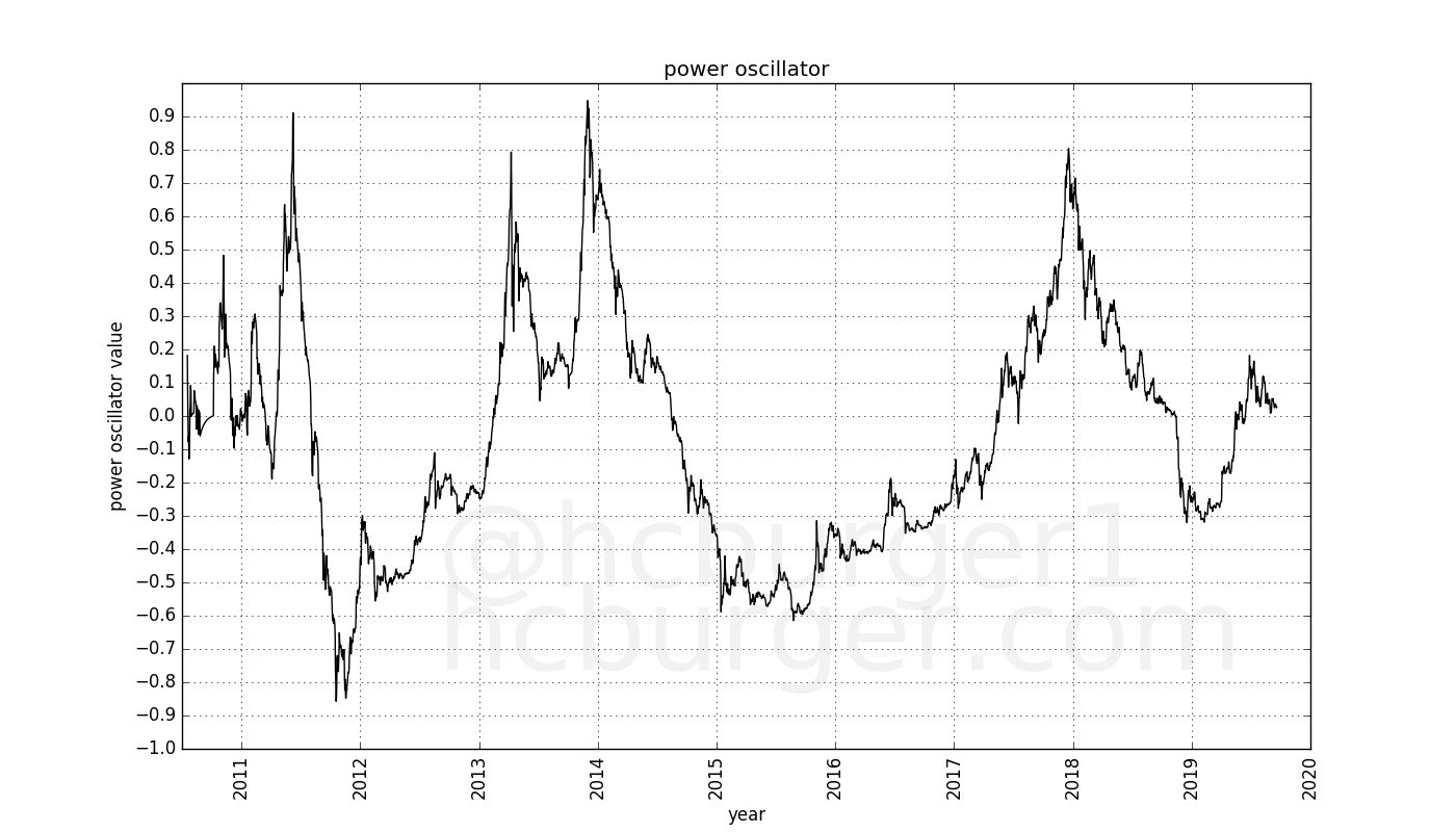
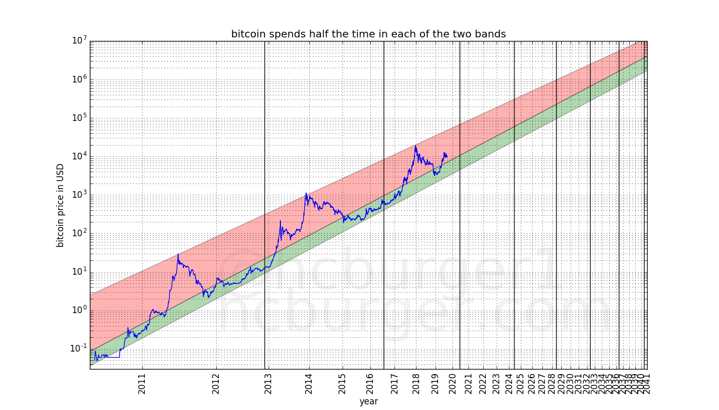
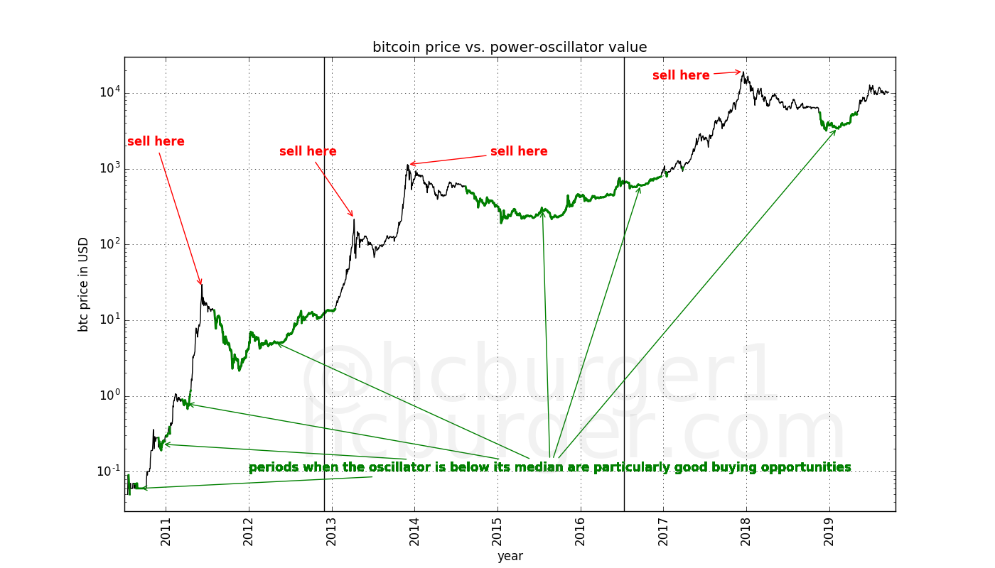
It moves approximately between -1 and 1 over time. If we color-code bitcoin’s price history with the oscillator value at the same time, we get the following chart:
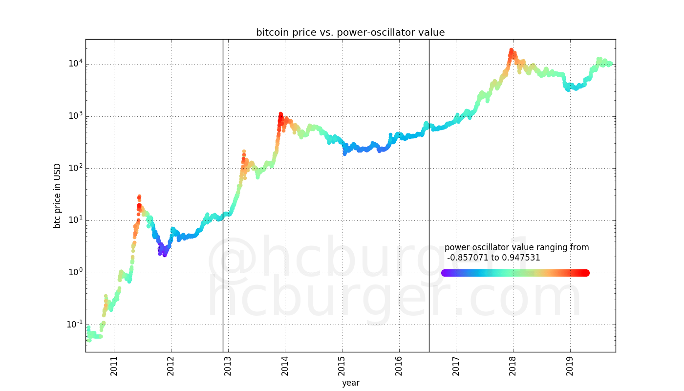
Market tops or all-time-highs coincide with high oscillator values perfectly. And market lulls coincide with lower oscillator values. Indeed, all four all-time-highs were achieved in a narrow oscillator band. These bubbles popped shortly after reaching that band.
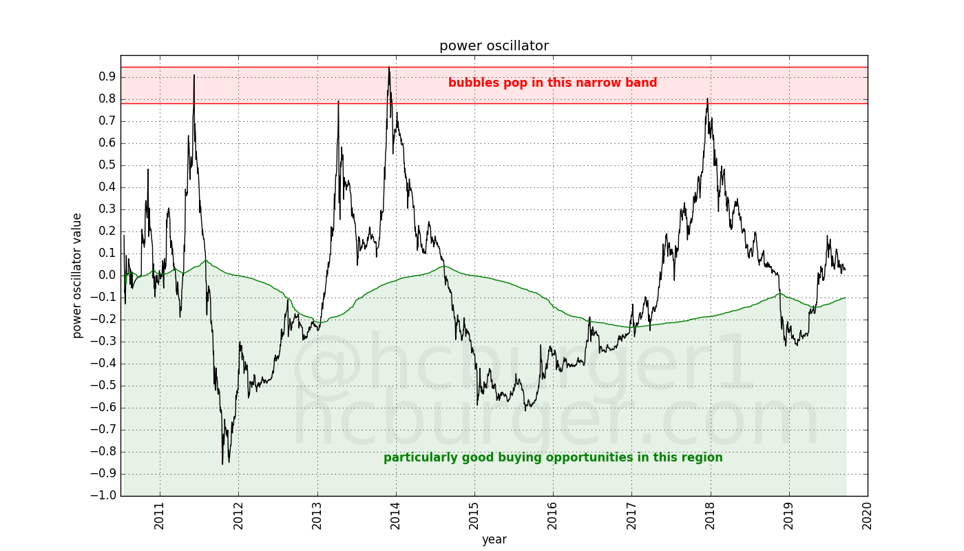
The green region describes the lower region in which the oscillator spends half its time. These moments can be considered to be particularly good times to buy bitcoin. The oscillator therefore recommends the following buying and selling strategy:
Even though these recommendations are not a perfect trading strategy, it is remarkable that the oscillator catches the market tops so well: All four all-time-highs are caught. The market lows are also caught quite well.
In the article “Bitcoin’s natural long-term power-law corridor of growth”, we have seen that bitcoin’s price history looks very linear in a log-log plot. The support line looks very linear, and three market tops also seem to lie a on a straight line. The overall price evolution also looks linear even though there is some volatility, and a robust fit yields similar results.
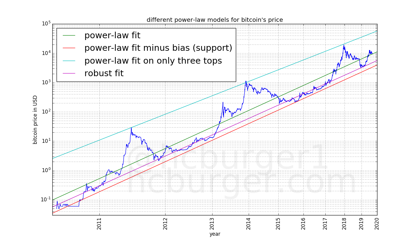
Straight lines in a log-log plot are in fact power-laws. Since the x-axis represents time, the power-laws are based on time. These lines can be projected into the future, leading to price predictions, which was the subject of the previous article:
What is interesting for this article is that the price moves within a corridor desribed by two power-laws. The intuition behind the oscillator described here is to look at where in the corridor the price is currently located.
The oscillator does not “cheat” because it only looks at the price information given at the time: it does not look into the future. This means that the oscillator value for the year 2014 does not assume knowledge of the bitcoin prices of 2015 for example.
Also, new market data does not change previously computed oscillator values. So no matter what the bitcoin prices will be in 2020 or beyond, the oscillator values that have already been computed will not change.
Since the oscillator is based on power-laws, we’re going to call it the power oscillator.
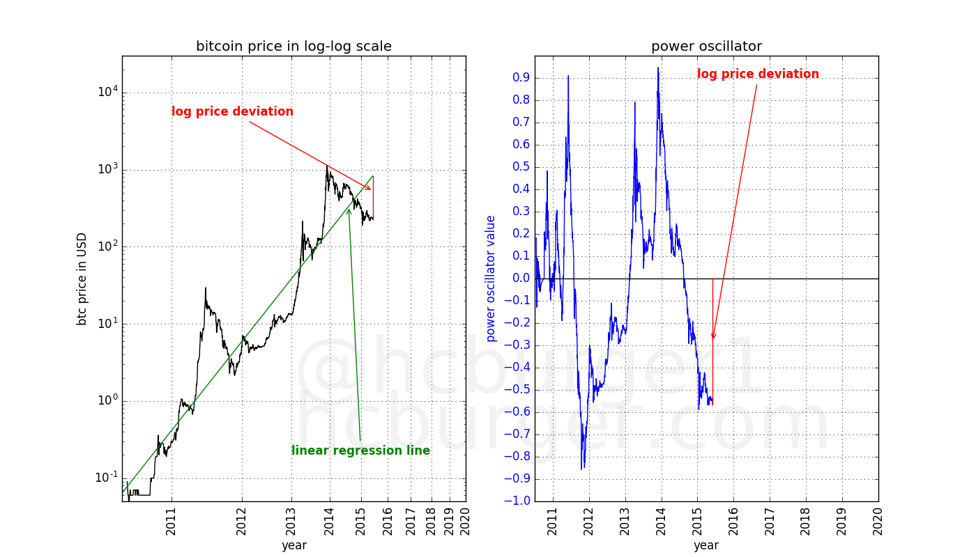
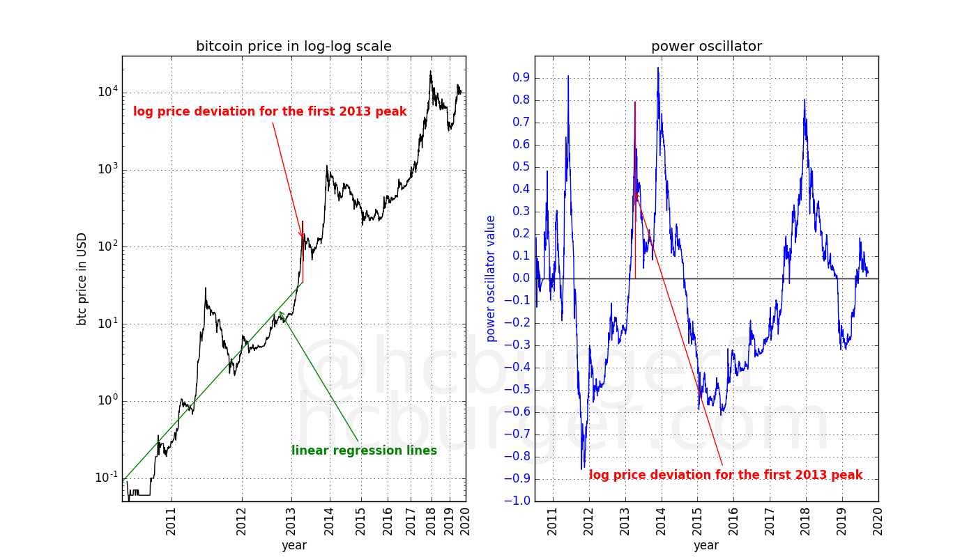
The power-oscillator is based on a linear regression of the price information in a log-log plot. This is the same principle as was used in the previous article. The below plot on the left shows bitcoin’s price history (in black) until the bubble of 2011, when it reached a price of approximately $30.
Linear regression is performed on this data, yielding the linear regression fit displayed in green. The deviation between the end of the price history and the end of the price fit is displayed in red: this is the log price deviation.
We take the length of this deviation and insert it into the plot on the right, for the same date. Since the actual price is above the price predicted by the linear regression fit, the devation is positive:
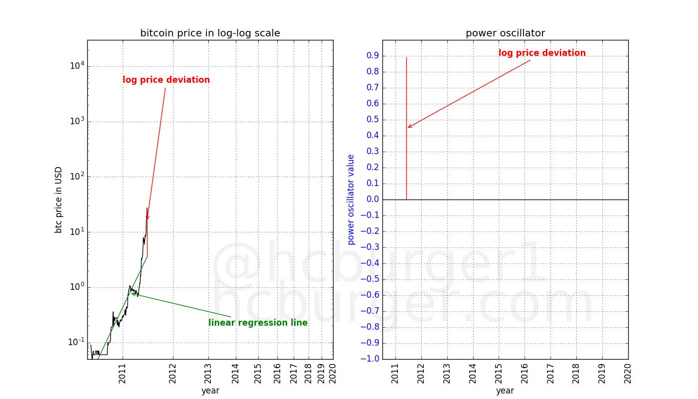
Note that only the price data available until 2011 is used. The regression is performed only on that data. Future prices are ignored because they are unknown.
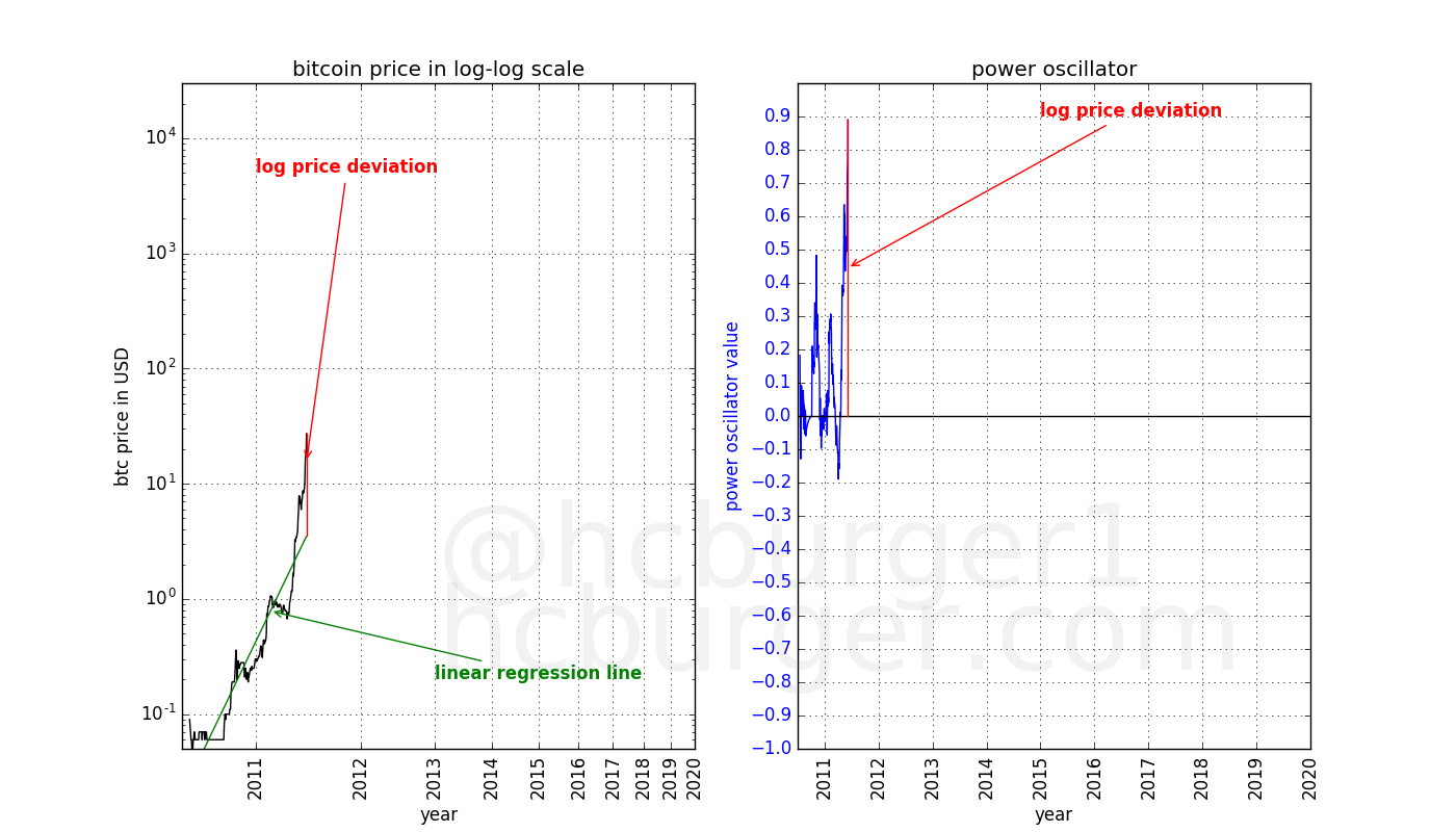
Had we performed the same procedure as above for each point in time until that date in 2011, and inserted a blue point in the graph for each log deviation, we would obtain the following figure:
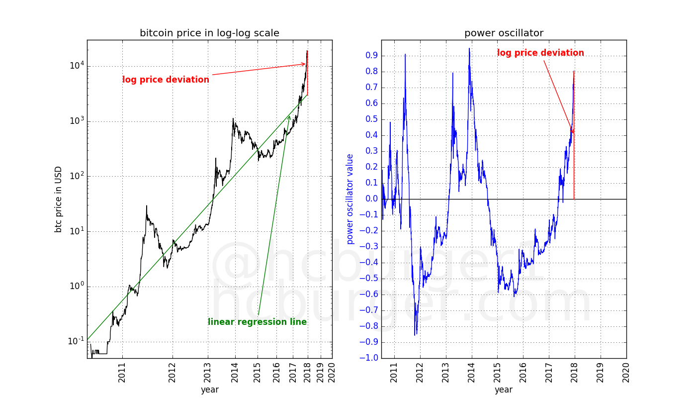
Let’s continue in the same fashion until mid-2015. Here the log-price deviation is negative because the actual price is lower than the price predicted by the linear regression model. Hence the oscillator has a negative value on that date:
Let’s keep going until the price peak achieved at the end of 2017:
And finally, let’s use all price data available to date. During this process of moving forwards in time, the oscillator values that have previously been computed have not changed. Current prices affect only the present oscillator value - past values are not changed.
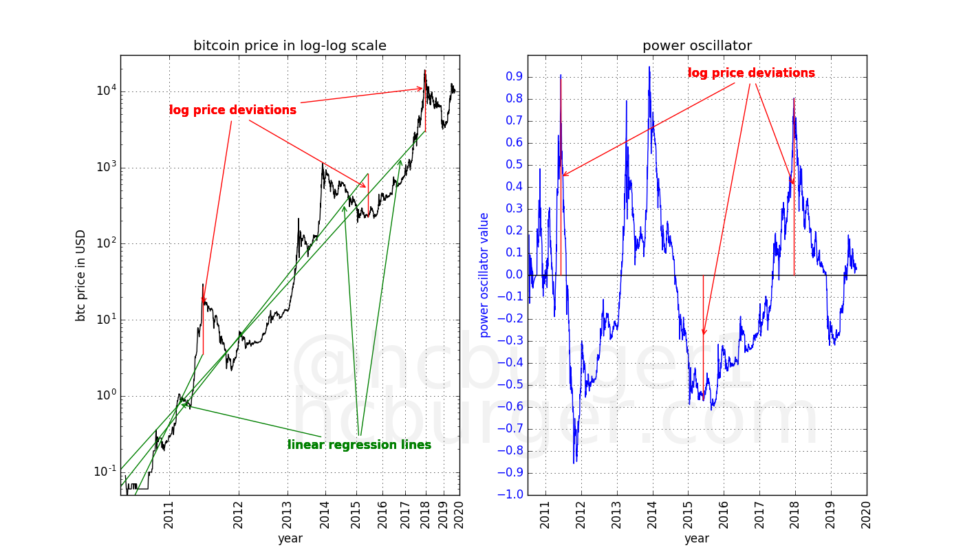
Super-imposed on the price data on the left graph we have the three different linear regression fits we obtained at the three timepoints we had chosen above. The linear regression models change over time: the slope can become larger or smaller. But only the log price deviations are used in the power oscillator.
The power oscillator up to the date of writing looks like this:
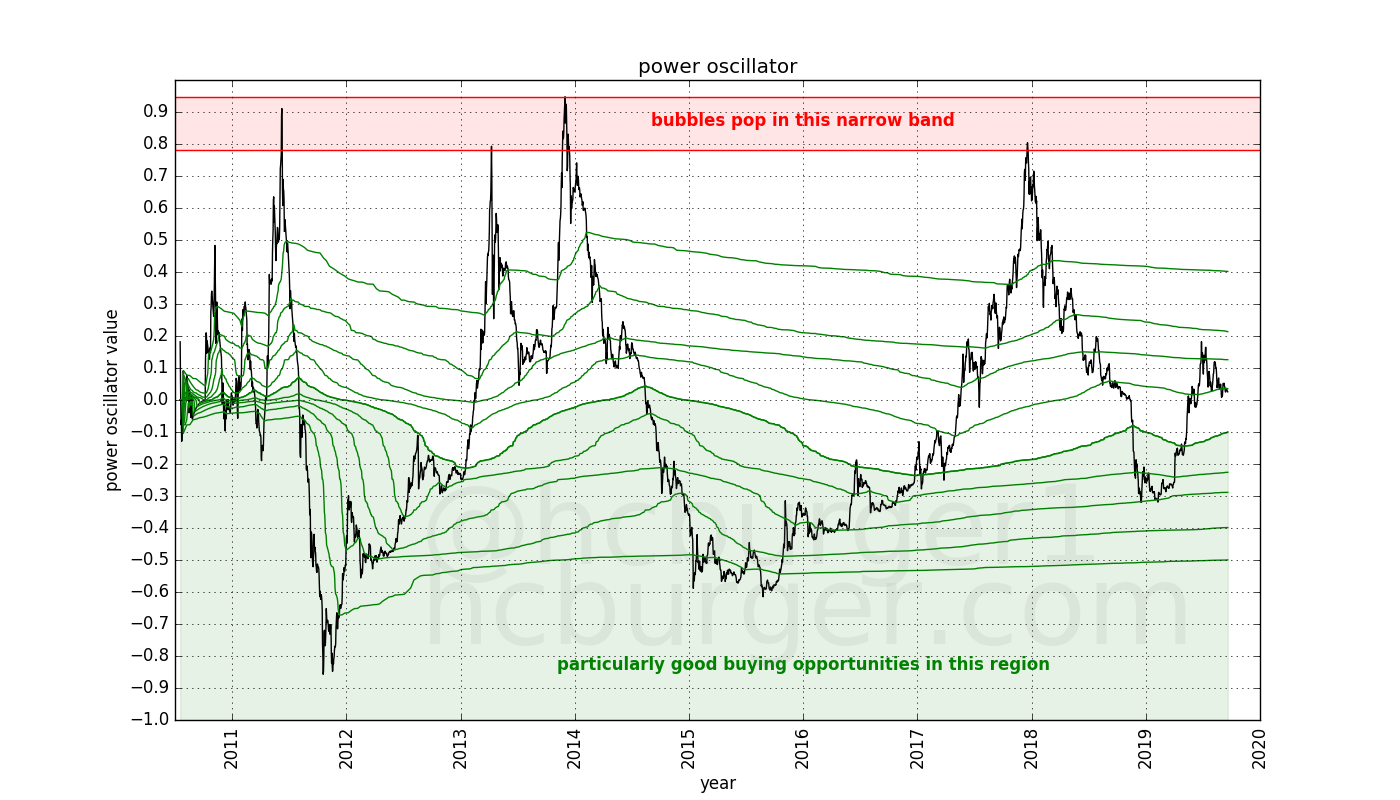
Low oscillator values indicate moments in time when the price of bitcoin is low compared to its long-term growth (power-law) trend. These moments should therefore present good opportunities to buy bitcoin. We will pick the moments were the oscillator is lower than the median oscillator as “good moments to buy”. We choose the median because it means that the oscillator spends half its time about this value, and half its time below this value. The median also has to be updated with time, since new data will influence its value. The green line in the plot below shows the median of the oscillator. Moments when the oscillator is below this curve can be considered particularly good times to buy:
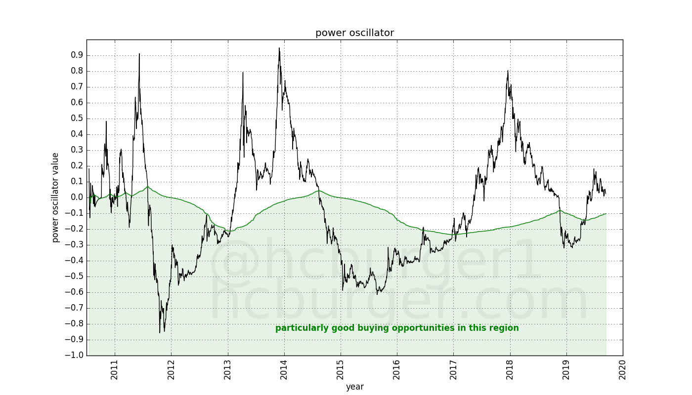
Using the median is also convenient because there is no need to hand-pick a certain threshold value, e.g. -0.1.
The reverse question is when to sell bitcoins. We notice that all four all-time-highs coincide with oscilator values that lie within a narrow band between about 0.8 and 0.9:
This is surprising. We have previously seen that three (not four) all-time-highs lie on a straight line in a log-log plot:
Two all-time-highs occurred in 2013, and only one of those lies on the top of the long-term price corridor. Yet, the power-oscillator catches this first bubble of 2013 as a market top.
Howcome? If we do a power-law fit to the bitcoin price data available up to the first 2013 bubble, we see that the price of the bubble indeed deviates significantly from the long-term fit of the time:
The fact that bubbles burst in the 0.8 to 0.9 oscillator band means that the market cannot support prices that are above a certain level above the long-term trend. If this threshold is breached, an abrupt downward correction occurs. Oscillator values of 0.8 to 0.9 correspond to a price that is about 6.3 to 8 times higher than the long-term power-law regression fit.
For the more technically inclined reader, in the below graph I have not only inserted the median, but also all other percentiles from 10 to 90 in steps of 10:
The power oscillator superficially resembles the Mayer mutiple. The Mayer multiple was proposed by Trace Mayer and compares the price of bitcoin to the 200-day moving average of the price. The Mayer multiple is the ratio between these two values: A Mayer multiple of 5 on day x means that the bitcoin price is 5 times higher than the 200-day moving average.
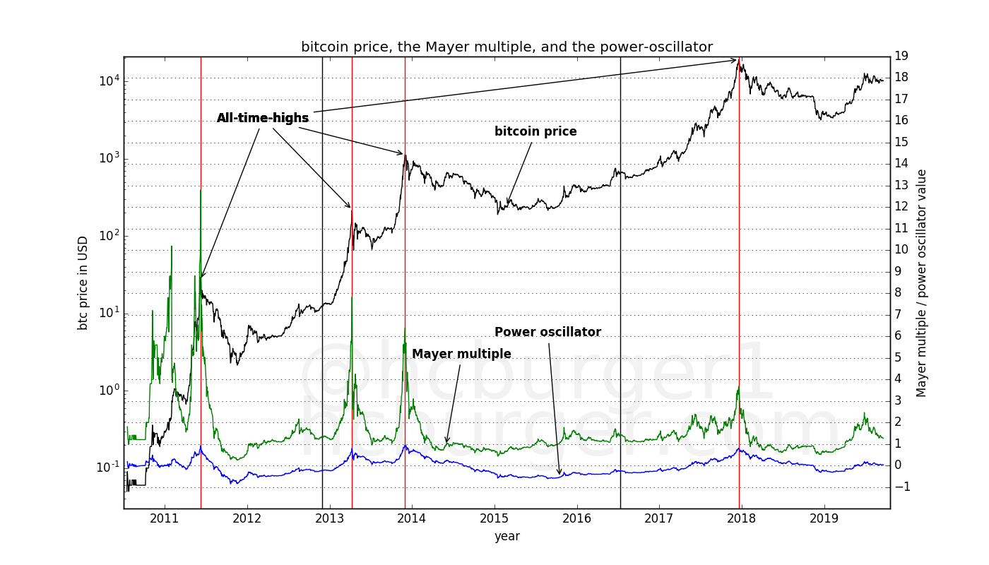
We immediately notice that the Mayer multiple and the power oscillator look superficially similar: they both achieve high values during market peaks, and lower values during market lulls.
However, an important difference is that the power oscillator has virtually the same value (0.8) at each all-time-high, whereas the Mayer multiple does not: It ranges between approximately 3.5 and 12 for the four different all-time-highs. The Mayer mulitple is therefore not as useful as the power-oscillator at timing all-time-highs.
It is claimed that it has been found that it is best to accumulate bitcoin when the Mayer multiple is below 2.4. Following this recommendation implies accumulating bitcoin during the green periods below:
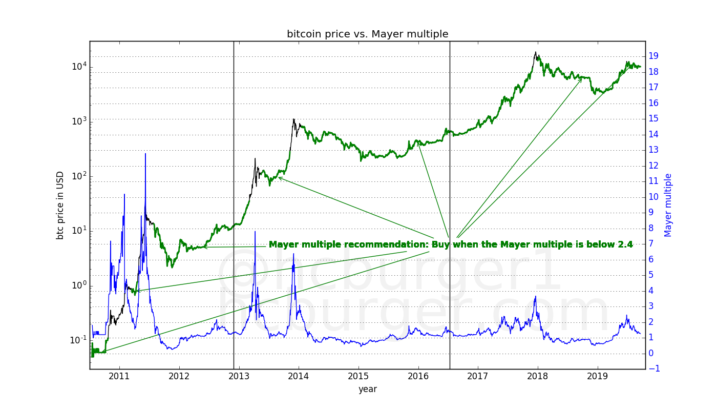
The results are not very convincing: the recommendation is to accumulate bitcoin at virtually all times. Such a strategy is unlikely to be the the best performing we can come up with.
An important difference between the Mayer multiple and the power oscillator is that the Mayer multiple depends on a manually chosen parameter: the 200-day moving average. It is not a priori clear why the choice of 200 should be the correct one. In fact, it is not clear that this parameter should not change over time, given that bitcoin’s price grows slower and slower over time.
The power oscillator has no parameter that needs to be manually chosen. It relies solely on the principle that bitcoin is likely to follow a power-law growth.
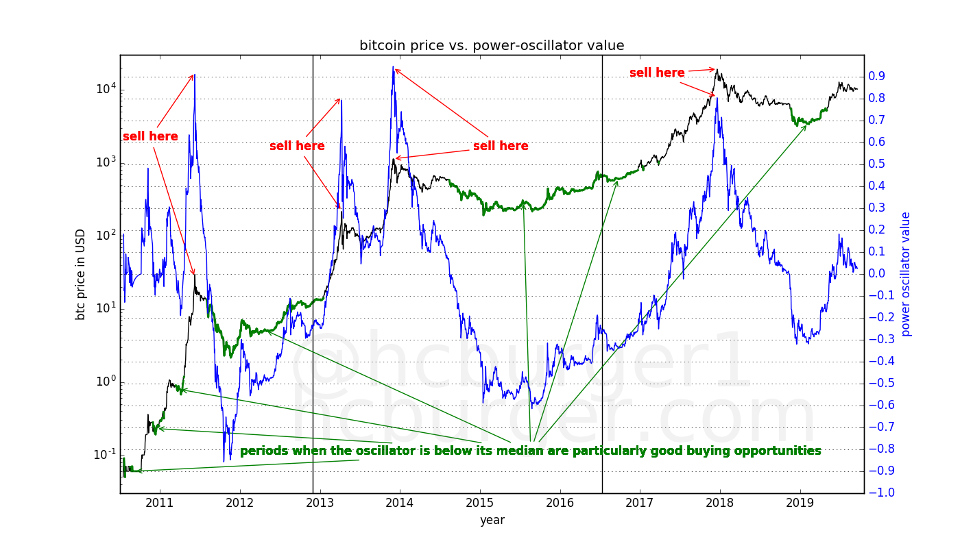
The above recommendations that flow naturally from the power-oscillator are summarized in the figure below:
To make the plot less crowded, let’s look at just the price data:
Let’s use these recommendations to devise a simple trading strategy where the investor:
Let’s compare this strategy to dollar-cost averaging, and let’s assume that the lucky investor does not have to pay taxes:

We see that the strategy guided by the power oscillator:
At first glance, it would therefore appear that the power-oscillator can be a useful tool in guiding a trading strategy. The threshold of 0.7 in this scenario was admittedly manually chosen, but it was also chosen to lie well below the usual value at which bubbles burst, so as to make the strategy more robust.
The above strategy is certainly not perfect. For example, there is no buy recommendation after the first sell recommendation during the first bubble of 2013. The next buy recommendation came at a much higher price than the peak of the first 2013 bubble.
Another imperfection is that the model seems to recommend to buy somewhat too early after a bubble.
Other trading strategies can certainly be divised using the power-oscillator (e.g. based on other thresholds or percentiles), but the goal of this article is not to find a perfect trading strategy but to present a simple indicator.
We have a introduced the power oscillator, an oscillator which
Another way of saying that bubbles pop at a power oscillator value above 0.7 is to say that the market cannot sustain prices that are more than about 5 times (or ![]() ) higher than what the power-law based trend-line would indicate. This is another indicator that power-law models are natural to bitcoin’s price history.
) higher than what the power-law based trend-line would indicate. This is another indicator that power-law models are natural to bitcoin’s price history.
The same reasoning holds for prices that are too low compared to the long-term power-law trend, except that corrections occur more slowly.
High values of the power oscillator are only possible if the price of bitcoin rises quickly. It the price rises more slowly, the power-law estimate of the price has time to adapt, leading to smaller power oscillator values.
It is worth noting that the power-law oscillator is indeed expected to keep oscillating, as long as bitcoin’s price growth continues to follow a kind of power-law. Should bitcoin’s price growth accelerate instead of decelerate (as is the case with power-laws), the power-oscillator would keep growing.
The fact that the power oscillator indeed oscillates around 0 (instead of e.g. growing perpetually), shows that bitcoin’s price history continues to follow a power-law, instead of e.g. exponential growth.
No tool is likely to be the perfect tool for timing the market. The power oscillator is no exception. I remind the reader that this article is not financial advice. I am not recommending any position in this article.
I would like to sincerely thank BitcoinEcon for the numerous interesting exchanges we had, and the early feed-back he gave me when reading drafts of this article. Thank you very much!